|
SqueezeBrains SDK 1.18
|
|
SqueezeBrains SDK 1.18
|
There are some guides that explain some key aspects on how to use the SB library.
SB Library
SB GUI
The installation of the SB Library and of the SB GUI is performed with the self-installing package downloaded from the FaberVision website (https://www.fabervision.com/). The installation and update process is managed by the SB Maintenance Tool application which supports the following operations:
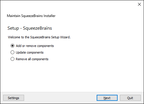
After the installation you will find the SB Maintenance Tool application in the installation folder, default ones are:
In case of a new SB SDK release or update a dialog will appear when opening the SB GUI informing that a new update is available. Select Update Manager in order to open a dialog that shows the updated packages highlighted. Select Update Now and then Yes in the following popup dialog. The SB Maintenance Tool will open showing the three installation options described before.
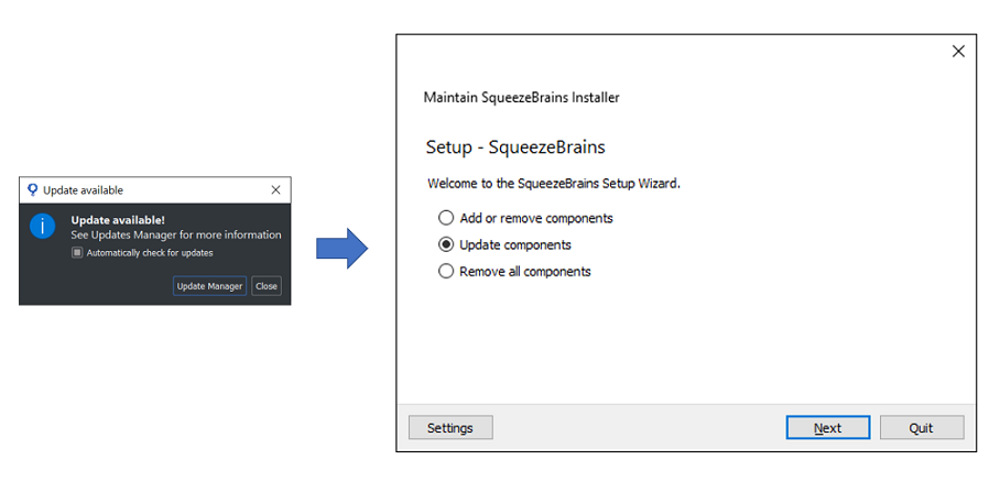
Choose the second option and in the next window select the packages to update and then confirm. At the end of the update you will be asked to Restart the Maintenance Tool.
In case a new SB SDK version is released and the update dialog does not pop up when opening the SB GUI or in case the installed version is less than 1.6 it is necessary to launch the SB_Maintenance_Tool.exe manually.
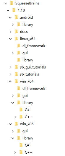
The following image shows how the SB components are organized in the repository installed by the SB Maintenance Tool.
The SB GUI is released for the following operating systems:
The SB GUI is installed with the SB Maintenance Tool with all the required dependencies.
The SB Library includes:
The SB dynamic library is:
In the following the compiler used and the dependencies:
The SB Deep Learning Framework is released for the operating systems Windows and Linux 64 bit.
During the installation procedure, if the detected operative system is compatible, the package is checked by default and its content is installed in the folder "dl_frameworks" located inside the installation folder of the specific SB SDK version. In case it is not installed, install it with SB_Maintenance_Tool .
SB Deep Learning Framework is a module containing all the dependencies necessary to run training and detection with SB deep learning modules, i.e. Deep Cortex and Deep Surface.
All deep learning algorithms and functions developed by FaberVision team are contained in the following extension libraries:
If the SB Deep Learning Framework is not installed it will be still possible to manage and perform basic operations on Deep Cortex and Deep Surface projects, e.g. creating a project, setting parameters, doing labeling and so on.
In the following the list of library dependencies included in SB Deep Learning Framework:
SB Deep Learning Frameworks include also a folder "dl_frameworks\pre-training" with a set of pre-training parameters configurations to use for facilitating the training.
The SB Library is released together with a C# Wrapper that could be useful in case the library needs to be integrated inside a C# .NET Application. The Wrapper is contained in the sb_cs.dll and it is contained in the same folder of the sb.dll.
The following list shows the main classes of the C# Wrapper:
For a quickstart guide see the C# Tutorials section
A SB solution is based on two main file formats:
the image information file (with an extension SB_IMAGE_INFO_EXT), one for each image of the dataset. It contains:
See Management of information relative to an image for more information.
So the files of a project are:
Regarding the location of these files you have full freedom apart from a single constraint: all the images used by sb_svl_run for training must be located in the same folder.
This folder is set by the parameter sb_t_svl_par::project_path and must contain also the rtn files of the images.
You have also to specify the extensions of the image to be used for the training with the parameter sb_t_svl_par::image_ext.
The same folder could also contain images used for test or actually not used.
You can specify which images are used for training, for testing and not used calling the function sb_image_info_set_type.
An image without the rtn file is considered as not used by default.
You could put the solution file rprj in the same folder or everywhere you want.
You can specify the folder of the rprj file when you call the function sb_project_load .
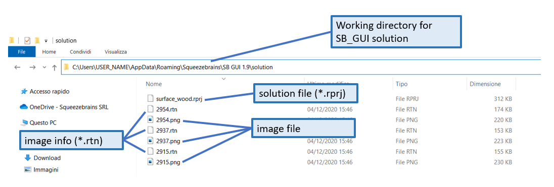
The SB GUI, for simplicity, puts the rprj , rtn files and images files in a folder named "solution" located at:
This working directory is fixed and cannot be changed.
However the user is free to save the current solution to any location on the disk as a ".zip" file. Note that each time a ".zip" solution is loaded from the SB_GUI all its contents is copied in the working directory and all the changes will interest only the files in the latter folder. In order to make the changes effective on the zip file the user need to manually press on Save Project / Save Project As.
In the following image it is shown the contents of the SB GUI working directory of the example solution "surface_wood.rprj".
In the following a brief description of all the possible functionalities and applications using the modules of SB SDK.
Object Detection means that computer vision technique used to locate instances of objects in digital images.
Instances can belong to different models, have different size and scale and be not limited in number. Also instances that are not entirely visible because covered, overlapped with other instances or partially outside the image are detectable.
In general, a few dozen of training images are enough to reach optimal results.
For this functionality is possible to use the following SB modules:
Image Classification means that computer vision technique used to assign a model (or a class) to an entire image depending on its content. The content to classify may be the whole information contained in the image, but also a part of it (as an image of an industrial component). The only SB module working for this functionality is Deep Cortex. It uses deep learning algorithm to classify an image returning a weight (i.e. a confidential score) for each possible model associable to it.
Anomaly detection means that computer vision technique used to examine an image and to detect those occurrences that are different (the "anomalies") from the established pattern learned by the algorithm (the "good" part). It usually involves unsupervised or semi-unsupervised training. SB SDK does not include yet a module specially designed for this purpose, but similar results are obtained by the following modules:
OCR (Optical Character Recognition) is the computer vision technique used to distinguish letters or text inside digital images. This technology is already widely applied to automatically read papers or digital documents, but it finds application also in other fields as industrial manufacturing, where reading characters or codes differently printed on various objects and surfaces is often necessary. However, traditional OCR are not able to work in this situations.
SB SDK provides to the user the Retina module to solve the problem. Given that Retina is an object detector, it is possible to associate each character to be found to a model and and treat as an object detection problem. Detected characters are grouped into strings according to their relative spatial location. The fact of not having any a priori-knowledge about characters feature therefore is an advantage. The algorithm specializes itself only on the characters provided by the user and is able to guarentee robustness to all that phenomena that characterized not digital written characters, such as distortions, discontinuity, blurring and so on.
Another advantage is that it can be trained to recognize special characters, such as symbols and logos, that are not contained in any pre-trained ocr algorithm.
Defect segmentation is the computer vision technique used to locate, classify and segment (detecting the boundaries) different models of defect on surfaces in digital images. It can be considered as a particular application field of the more generic family of Semantic segmentation algorithms. The segmentation of the defects is usually done at pixel level. The contributions of all the pixels are combined in order to form a vote plane. Only later all the pixels that are classified with the same "defect" and are contiguous are merged together in a blob representation.
SB SDK includes the following built-in modules to solve defect segmentation tasks:
Instance Segmentation is the computer vision technique that involves identifying, segmenting and separating individual objects within an image. It's similar to Defect segmentation with the only difference that contiguous pixels that belong to different object instances are not merged together. Therefore it allows to segment and separate partially overlapped object.
SB SDK does not include yet a module specially designed for this purpose, but in case of separated objects we may consider Surface and Deep Surface modules working as instance segmenters.
Keypoint location is the computer vision technique used to locate peculiar points or spatial features of an object inside the image. These points usually are invariant to image rotation, shrinkage, translation, distortion, and so on.
SB SDK does not include yet a module specially designed for this purpose, but is possible to train Retina module to detect a characteristic parts of an object. To reach this objective may be useful to run different Retina tools in cascade, where the first used to locate the object and the later to find the keypoint on it.
In the major of the applications Retina is applied to solve object detection problems using a supervised approach. Supervised learning consists in training a classifier using a dataset in which the target of the detection task is "well" labeled and the algorithm learns to generalize about the object from the object instances provided by the user.
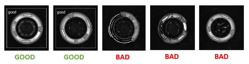
However, Retina demonstrates to reach good results even used in a semi-supervised manner. Let suppose that our objective is to distinguish between good and bad pieces at the output of a stage in a production line. We have no idea about what kind of defects may appear on the object: the only information that we can provide to the classifier is if a given piece is good or not. Such approach is defined as semi-supervised learning, because the system is able to identify a reject using only good pieces marking as "bad" whatever piece does not produce a detection.
Here, some guidelines for an semi-supervised use of Retina to sort good and bad samples follow:
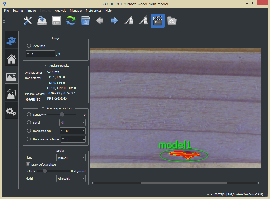
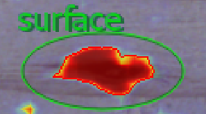
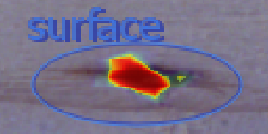
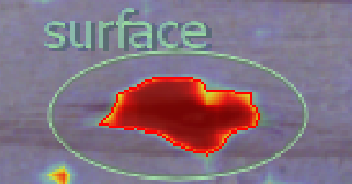
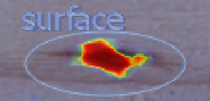
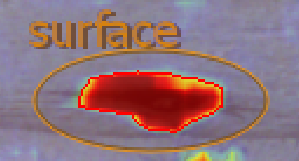
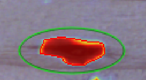
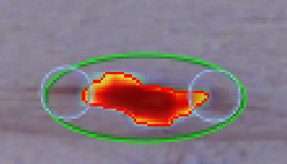
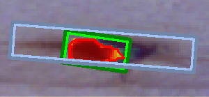
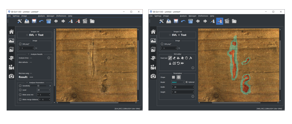
In the following images an example of semi-supervised use of Retina for sorting good and bad samples. In this case, the objective is to identify defects on the orange socket of the metal valve and in the central hole. Model "good" is associated only to those samples with no defects. The training results visible from the weight maps are quite satisfying: the classifier has learned to well distinguish between good and bad pieces providing also useful information about the defect position (marked in red).

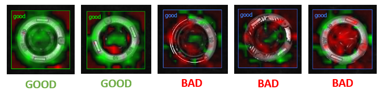
The SB Library includes four modules divided in two categories:
The figure below graphically shows the relation between Shallow Learning and Deep Learning algorithms in relation to Artificial intellligence.
The main characteristics of SqueezeBrains modules are summarized in the following table:
| Characteristic | Supporting modules | Description | |||
|---|---|---|---|---|---|
| Retina | Surface | Deep Cortex | Deep Surface | ||
| It simulates the human vision perception system | ✔ | ✔ | ✔ | ✔ |
|
| Generic analysis not dedicated to any specific task | ✔ | ✔ | ✔ | ✔ | Many artificial intelligence algorithms are designed to work only on specific vision tasks. Think, for example, to "faces recognition" or "vehicle detection" systems used in security or in automotive industry: they represent the state-of-art of the available technology in those sector, but their applications are extremely limited. All SqueezeBrains modules overcome these limitations because are able to extract generic information from images which may fit to different vision applications. |
| Reduced number of configuration parameters | ✔ | ✔ | ✔ | ✔ | SqueezeBrains modules are designed in order to be user-friendly. This implies a reduced number of configuration parameters that user have to set. In more detail:
|
| It learns through the training | ✔ | ✔ | ✔ | ✔ | With traditional analysis, for each vision problem to be solved, a sequence of fixed operations must be defined. Instead, machine learning techniques allows to have a library that automatically learns what to do. In the case of Retina or Deep Cortex they learn the characteristics of the object/objects in the image, in the case of Surface or Deep Surface they learn the defect to be found. |
| Reduced number of images | ✔ | ✔ | ✖ | ✔ | For most of applications, few tens of training images are enough to reach optimal results. The only module that requires an higher number of images is Deep Cortex. |
| Supervised learning (SVL) with human-machine interaction | ✔ | ✔ | ✔ | ✔ | Learning begins with a small set of images. Then the labeling assistant function of the SB GUI helps the operator to do the labeling: the system proposes and the operator confirms, and if there is an error the operator corrects it and adds the image to the training dataset. In this way it quickly reaches a stable learning ready to be used in the machine.
|
| Multi-models management | ✔ | ✔ | ✔ | ✔ | It is possible to create multiple models to associate to different objects/defects in the same project. Each model can be enabled/disabled independently during the detection phase. |
| User scale management | ✔ | ✔ | ✖ | ✖ |
|
| Optional samples and defects | ✔ | ✔ | ✖ | ✔ | Being able to declare a sample or a defect as optional allows you to handle those cases in which even for user it is difficult to understand whether that sample is good or bad, whether that defect is actually a defect or is a good part. Optional samples/defects are not used for training and do not affect statistical indices such as accuracy. For optional samples/defects two special classes have been defined called Optional Positive and Optional Negative depending on whether the predicted weight, or confidence, is greater than or equal to 0 or less than 0.
|
| Collaborating models management | ✔ | ✔ | ✔ | ✔ | Collaboration between models allows you to correctly manage cases in which you have models of objects that, because of their variability, can become very similar to each other. In this case, it is advisable to set up these models as collaborating to improve detection results. In Retina and Surface collaborating models are used also in training phase. |
| Support for multi core processing | ✔ | ✔ | ✔ | ✔ | It is possible to set the maximum number of CPU cores that the library can use for training and image processing.
|
| GPU is not mandatory | ✖ | ✖ | ✔ | ✔ | Contrary to the majority of existing machine learning software, the use of GPU NVIDIA is not mandatory. Retina and Surface tools works only on CPU, while Deep Cortex and Deep Surface can works both with CPU and GPU NVIDIA. In the latter case GPU NVIDIA is strongly recommended only for training phase.
|
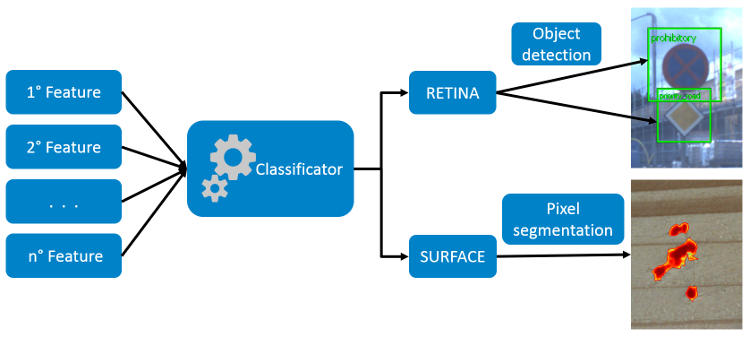
This section briefly describes how Retina and Surface works.
Both the modules are based on the same algorithms, but they differ in the format of the output results: Retina returns coordinates of the occurrences of the objects found, while Surface returns a voting plan.
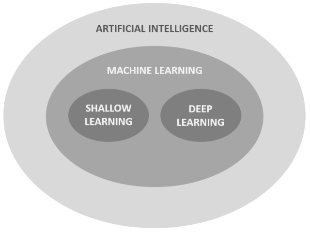
The approach used is that of the Sliding Window. The window always has the size of the model defined with the sb_t_par_model::obj_size parameter. To reduce calculation times, the model window is scrolled on the image with a scan step, which is predefined and equal to 4 pixels in Surface projects, while, in Retina projects it is defined by the variable sb_t_par_model::obj_stride_coarse. In Retina projects, if in a point of the image the probability that there is an object increases then, in the neighborhood of the point, a finer scanning step, defined by the variable sb_t_par_model::obj_stride_fine, is used.
The scale is managed as follows: the image is scaled while the model remains of the original size.
The model window is moved on the image and in each position the features are extracted and assembled in a data vector.
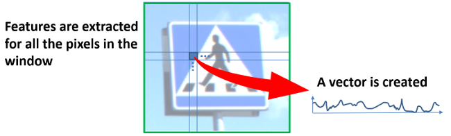
The sb_svl_run training function automatically chooses the best features but it is still possible: 1) to set the features from which it choose automatically or 2) manually choose the features that the training must use. See the guide features for more information about the features and their selection. In each position of the scan grid of the window on the image, the vector of the features is calculated and sent to a classifier to predict the presence of the object or defect. So the prediction generates a confidence or weight value that has a value between -1 and 1.
The minimum dimension of an object or a defects is 8x8 pixel.
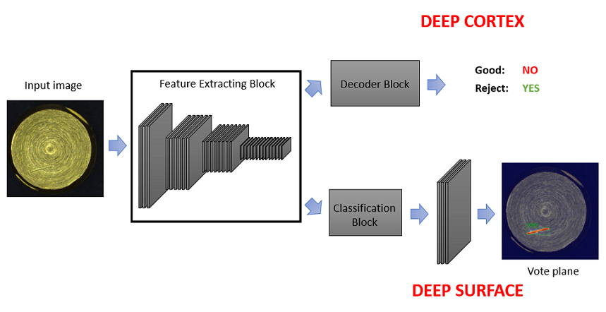
This section briefly describes how Deep Cortex and Deep Surface works.
Deep learning modules developed by FaberVision are all based on Convolutional Neural Networks (CNN) architectures. The core of these algorithms is the Feature Extracting Block (also called Backbone or Encoder) which is responsible for the following operations:
Feature maps at the output of the backbone are used to fed a processing block which differs according to the project type:
In the following image a simplified blocks diagram of SB deep learning algorithms is reported.
The result of the analysis of Retina project is a list of samples with the following properties:
The result of the analysis of Deep Cortex project is a list of samples with size equal to sb_t_par_models::size. Each sample contains the classification result of the image for a specific model of the project. The order policy of the samples returned by sb_project_detection function may differ according to the following conditions:
| ground truth | almost a sample with weight > 0 | criterion order |
|---|---|---|
| no | yes | descending order of weight |
| yes | yes | descending order of weight |
| yes | no | first sample with the same model of the ground truth (FALSE NEGATIVE), others in descending order of weight |
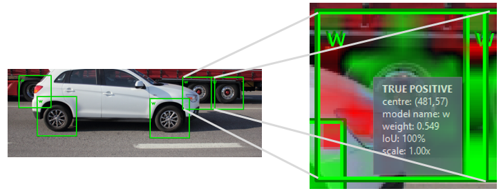
Each sample is completely described by the following properties:
To facilitate a graphical representation, centre and vertices of the sample are set in such a way that sample has the same size of the image to classify.
The main result of the analysis of Surface or Deep Surface project is the segmentation.
The function sb_project_detection calculates:
Moreover the function sb_project_detection calculates a blob analysis on the voting plane in order to group defects areas with same models and allow you to filter out the defects based on various criteria of form and proximity (see blob analysis parameters). You will find the list of the blobs with their properties in the struct sb_t_surface_res . See sb_project_detection to learn how to enable the blob analysis.
The function sb_project_detection calculates more properties if the ground truth or labeling has been passed to the function, in particular:
The following table summarizes the truth value (TP, FP, FN, TN, OP, ON) expected output given the ground truth/labeling and the defect occurrence found.
In the images of the Ground truth / Labeling in the tables below with the red color you can see the required defects and with the brown color the optional defects.
| Ground truth defect area | Optional? | Occurrence defect area | Truth value | Ground truth/Labeling | Result |
|---|---|---|---|---|---|
| area >= sb_t_blob_par.area_min | NO | area >= sb_t_blob_par.area_min | TP | 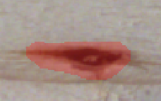
| 
|
| area >= sb_t_blob_par.area_min | NO | area < sb_t_blob_par.area_min | FN |
| 
|
| area < sb_t_blob_par.area_min | NO | area < sb_t_blob_par.area_min | TN | 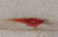
| 
|
| area < sb_t_blob_par.area_min | NO | area >= sb_t_blob_par.area_min | TP |
|
|
| area >= sb_t_blob_par.area_min | YES | area >= sb_t_blob_par.area_min | OP | 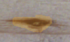
| 
|
| area >= sb_t_blob_par.area_min | YES | area < sb_t_blob_par.area_min | ON |
| 
|
| area < sb_t_blob_par.area_min | YES | area < sb_t_blob_par.area_min | ON | 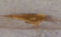
|
|
| area < sb_t_blob_par.area_min | YES | area >= sb_t_blob_par.area_min | OP |
|
|
| NO defect | NA | area >= sb_t_blob_par.area_min | FP | 
| 
|
| NO defect | NA | area < sb_t_blob_par.area_min | TN |
|
|
Regarding the required and optional ground truth areas, there are two different situations that may happen and lead to an additional OP/ON results or not.
See the following table:
| Situation | Truth | Ground truth/Labeling | Result image |
|---|---|---|---|
| The occurrence blob overlaps both the required and the optional ground truth blobs | 1 TP | 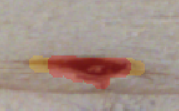
| 
|
| The occurrence blob overlaps only the required ground truth blob | 1 TP and 2 ON |
| 
|
| The occurrence blob overlaps only the required ground truth blob and the merge distance is large enought to merge the ON blobs | 1 TP and 2 ON |
| 
|
Image results
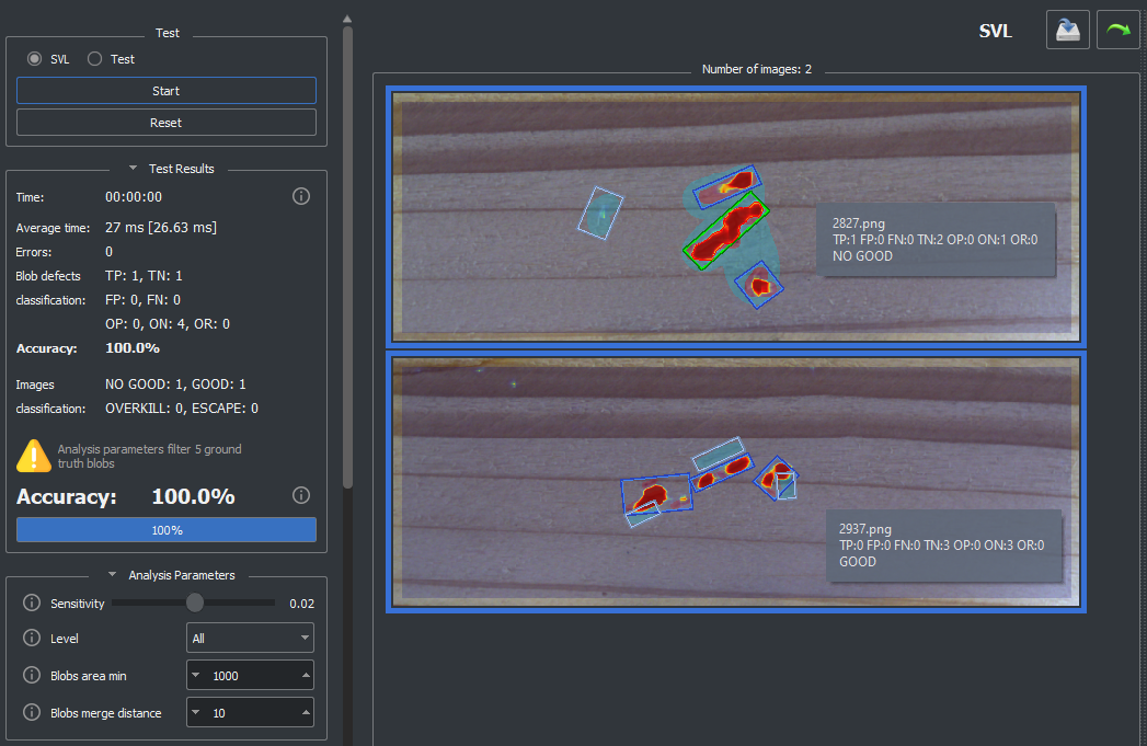
In the results of image detection the TN blobs are always counted both in the global results and in those per model.
Furthermore, the TN counter in the global results is set to 1 if there are no TP, FP, FN blobs in the image.
Statistics / metrics
In statistics, the counting of TN instance follows a different logic in order to have metrics that are more meaningful.
The TN counter of the models is always set to 0 while the TN counter of the global increases by 1 for each image without any TP, FP and FN blobs. The same convention is also used in Retina projects.
Example
Let's consider the case of a project with two models, 'a' and 'b', 100 test images and only one of these images has a defect of model 'a', furthermore we assume that we have no FP blobs.
The statistics of the model 'a' are different depending on whether:
Therefore in the first case the accuracy of the model 'a' is equal to 0% while in the second case it is 99% with the consequence that the FN is "hidden" by the TN counters.
This way of counting the TN in the statistics allows the metrics to "focus" on the images in which the defect is present while neglecting the others.
The image below shows the case of two images: the sb_t_stat_model::tn counter of the global result is 1, because there only 1 image that has no TP, FP and FN blobs, while the sb_t_res_model::tn counter is equal to 2 for the first image and equla to 3 for the second one.
In this section the naming of the SB library is explained.
Naming convention of the functions of the library is:
For example: sb_project_get_par where "sb_project" is the acronym, "get" is the action and "par" is the object.
When defining a function, the order of the parameters is usually: input, then output. For example the function sb_project_get_stat .
But if the fuction returns an SB_HANDLE then the handle is always the first parameter of the function, for example sb_project_load .
the acronym is formed as follows: sb _ name of the class.
In the following the list of the acronyms of the SB library:
Some typical actions are in the following table:
| action | example |
|---|---|
| create | sb_lut_create |
| destroy | sb_image_destroy |
| format | sb_license_format_info |
| get | sb_project_get_par |
| set | sb_project_set_par |
| load | sb_project_load |
| clone | sb_project_clone |
| save | sb_project_save |
| add | sb_par_add_model |
| remove | sb_par_remove_model |
Some typical objects of the action are in the following table:
| object | example |
|---|---|
| sb_t_version | sb_solution_get_version |
| sb_t_info | sb_project_get_info |
| sb_t_res | sb_project_get_res |
| sb_t_stat | sb_project_get_stat |
| sb_t_par | sb_project_get_par |
| sb_t_par | sb_project_set_par |
Types like structures or enumerators are always in the form: sb_t_ followed by the name of the class, for example sb_t_par or sb_t_project_type.
If the structure has a sub type the name has the following format: sb_t_ type _ subtype , for example sb_t_par_models.
The SB Library is based on "handles" which are objects with type SB_HANDLE.
An "handle" is a "black box" object and can only be managed with functions.
The handles of the library are the following:
The handles project and image information are threads save.
The SB Library has also many other objects that are structures. The main objects are the following:
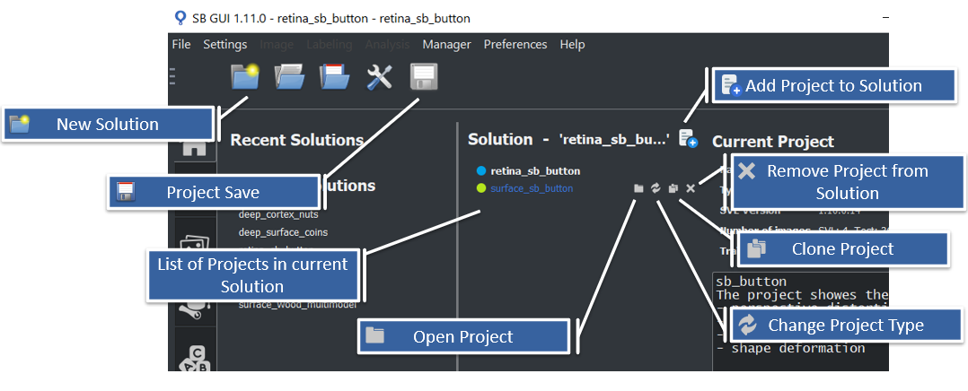
In this section the main operations on a solution and its projects are described.
With solution we mean a file, created by the library, which contains one or more projects of different type. The solution files created with the SB GUI have the extension rprj, but the user can use the extension he prefers. Basic operation for managing projects in a solution are the following:
At any time is possible to have access to general information about a solution by sb_solution_get_version and sb_solution_get_info functions. Especially the latter is useful because, among other information, returns the current active project of the solution. The user can modify this value calling sb_solution_set_current_project function. For more details see Solution structure.
All these operation are fully integrated in SB GUI in order to facilitate the user to manage solution and its projects. Figure below shows the basic graphic utilities to perform all the operations. Note that in SB GUI, every change to solution structure is automatically saved in the corresponding rprj file.
The following chapters show how to manage a solution file and projects with SB Library.
To create a project you should call the function sb_project_create.
In the example below you can see the creation of a new Retina project named "retina_project"
Instead of SB_PROJECT_TYPE_RETINA you can use SB_PROJECT_TYPE_SURFACE or SB_PROJECT_TYPE_DEEP_SURFACE or SB_PROJECT_TYPE_DEEP_CORTEX to create a project of different type.
To save a project in a solution you should call the function sb_project_save.
In the example below you can see the saving of a project handle in a solution named "example_solution.rprj"
To set the project as the current project of its own solution you should call the function sb_solution_set_current_project.
In the example below you can see setting a project as the current project of its own solution.
sb_handle is a project handle previously loaded with the function sb_project_load or created with the function sb_project_create.
To load a project from solution you should do the following operations:
To clone a project you should call the function sb_project_clone.
In the example below you can see the cloning of a project handle already loaded in memory. New project uuid is assigned to the new clone project.
sb_handle is a project handle previously loaded with the function sb_project_load or created with the function sb_project_create.
To remove a project from solution you should call the function sb_solution_remove_project.
In the example below you can see the removal of the j-th project module from "example_solution.rprj" file.
To destroy the solution info structure you should call the function sb_solution_destroy_info
To set parameter in a project you should do the following operations,
where sb_handle is a project handle previously loaded with the function sb_project_load or created with the function sb_project_create :
To enable/disable a model of the project you should do the following operations,
where sb_handle is a project handle previously loaded with the function sb_project_load or created with the function sb_project_create :
To add a model to a project you should do the following operations,
where sb_handle is a project handle previously loaded with the function sb_project_load or created with the function sb_project_create :
To remove a model from a project you should do the following operations,
where sb_handle is a project handle previously loaded with the function sb_project_load or created with the function sb_project_create :
To elaborate an image with a trained project you should do the following operation (See also tutorial_3_retina_detect),
where sb_handle is a project handle previously loaded with the function sb_project_load or created with the function sb_project_create :
To get the statistics related to the last processed images you should do the following operations,
where sb_handle is a project handle previously loaded with the function sb_project_load or created with the function sb_project_create :
You can store your own custom parameters both in a project and in a SB_IMAGE_INFO_EXT file. The information are save in xml format.
To load the custom parameters use the function sb_project_get_custom_par_root.
sb_handle is a project handle previously loaded with the function sb_project_load or created with the function sb_project_create.
To add a new parameter use the following function
To add a new structured parameter with sub-parameters use the following function
To remove a parameter use the following function
To set the value of a parameter use the following function
To get the value of a parameter use the following function
To get the xml node of a parameter use the following function
Suppose you want to add the following custom parameters XML structure:
Please use the following code to get it,
where sb_handle is a project handle previously loaded with the function sb_project_load or created with the function sb_project_create :
Each image of the solution is associated with a file, called image information file, that contains all image information necessary for svl and detection. The file has the same name as the corresponding image but extension SB_IMAGE_INFO_EXT.
Image information file contains:
To manage the image information file it is necessary to call functions with the acronym sb_image_info (e.g. sb_image_info_load, sb_image_info_save).
All these functions work separately on a image information handle, which is associated to a single project contained in the image information file.
To add the image information related to a project image to an image information file you should do the following operations,
where sb_handle is a project handle previously loaded with the function sb_project_load or created with the function sb_project_create :
To add a sample to an existing image information handle you should do the following operations,
where image_info is a "image information handle" previously loaded or created with the function sb_image_info_load :
To set the roi to an existing image information handle you should do the following operations,
where image_info is a "image information handle" previously loaded or created with the function sb_image_info_load :
To reset image information related to a project you should do the following operations,
where image_info is a "image information handle" previously loaded or created with the function sb_image_info_load :
To clone an image information handle and write it to *image information file** you should do the following operations,
where image_info is a "image information handle" previously loaded or created with the function sb_image_info_load :
To remove image information related to a project from image information file you should follow the following operations,
where sb_handle is a project handle previously loaded with the function sb_project_load or created with the function sb_project_create :
In supervised machine learning application, image labeling is a fundamental operation having a strong influence over the goodness of the final results. Labeling is the procedure that consists of locating any sample or defect instance in the correct position over the image. It is (almost always) manually done by an user and for this reason may be a time-consuming operation, especially when involves a great number of images. Its importance is quite intuitive: once learning process is started, elaboration criteria are directly inferred from image data, without any user interaction. Thus, before to start any SVL it is necessary to have a training dataset labelled as accurate as possible.
You can do the labeling using the SB GUI.
To facilitate labeling, the Labeling Assistant has been developed in the SB GUI, see Labeling assistant with SB GUI for more information.
Below the labeling procedure for SqueezeBrains tools is described.
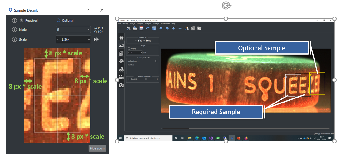
Labeling procedure for Retina projects is not particularly complex. After defining a new model, the user has to add a sample for each model occurrences into the image using sb_image_info_add_sample or sb_image_info_set_samples function. Each sample is a bounding box item and it is fully described by the information of the structure sb_t_sample . In the following some hints are reported in order to do a correct labeling:
In the figure below some of the previous points are graphically represented in SB GUI.
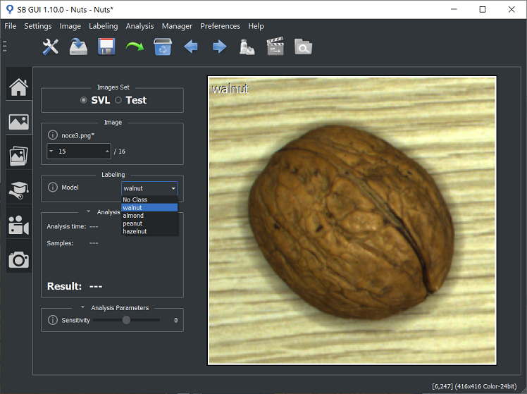
Labeling procedure for Deep Cortex is very simple. After defining a new model, the user has to set at most one sample to the image using sb_image_info_set_samples function. The sample describes the model associated to the image. If the image is not associated to any model, no sample has to be set.
Note that in a Deep Cortex project, information about sample position in the image is not important for training and inference. However, to facilitate the graphical representations of the sample over the image, it is advisable to set sb_t_sample::centre equal to the coordinates of image centre and sb_t_sample::scale = 1.0.
In the SB GUI it is also possible to select a group of images and set the model for all of them at once.
The figure below shows how to do labeling in SB GUI.
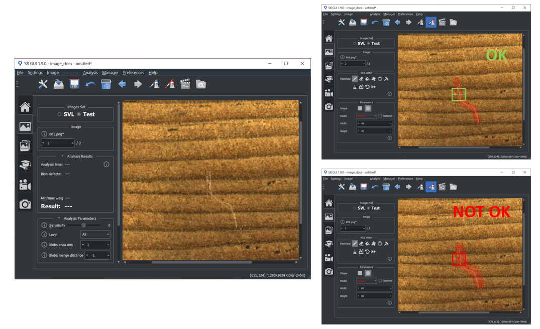
Labeling procedure for Surface and Deep Surface projects is more complex than Retina and Deep Cortex ones. This is because surface defects cannot be described and labelled as rectangular bounding boxes but requires a labeling that can perfectly fit to their shape and orientation at pixel level. Thus, defects are labelled over a ROI defects, which allows an higher degree of flexibility. ROI defects is set over the image using sb_image_info_set_roi_defects function. In the following some hints about how to mark ROI defects are reported:
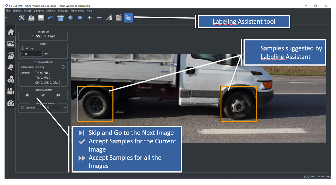
In order to facilitate and speed up data labeling procedure, SB GUI offers a Labeling assistant tool. This tool allows user to use the SVL training currently saved in memory for data labeling of unlabeled (or partially labeled) images. Labeling assistant graphically suggests for each image a list of sample/defect instances, that can be freely modified and then accepted by the user. However it is always necessary a careful supervision on the automatic procedure, because the classifier may commit mistakes, especially when the current training is not robust.
Image below shows the overview of labeling assistant tool in Retina, with its main operations.
To recognize objects and defects with Retina and Surface projects, a set of features is extracted from the image and classified. Available features are fixed and designed by SqueezeBrains. Generally the optimal feature set is automatically selected by the SVL, i.e. by the sb_svl_run function. The set of features is configured with the parameter sb_t_svl_sl_par::features, and is initialized with a predefined set of different features depending on the project type, Retina and Surface. See the table below.
| Project | Predefined set of features |
|---|---|
| Retina | 0A, 0B, 2A, 2B, 2C |
| Surface | 2A, 2B, 2C, 2A_R, 2AA_R, 2B_R, 2C_R, 2A_G, 2AA_G, 2B_G, 2C_G, 2A_B, 2AA_B, 2B_B, 2C_B |
Obviously it is possible to create your own set of features so as to condition the choice of the SVL.
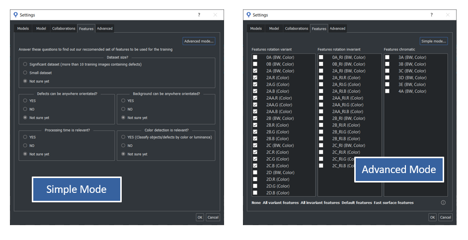
In the project settings menu of the SB GUI , it is possible to select the features in two different ways:
However, the set of features effectively used for the training, may varies according to the sb_t_svl_sl_par::optimization_mode parameter and to the type of images. For example, some features can only be used with BW images, others only with color images (RGB or BGR), and others with both BW and color images. Use the function sb_feature_description to get this information from the library.
The name of the features has the following format: 2A[A][_RI][.R].
The name is composed by the following elements:
The following table lists the features and their characteristics.
| Name | Image format | Description |
|---|---|---|
| Category "0" | ||
| 0A 0B | BW RGB BGR | The feature is sensitive to the transitions between light and dark and viceversa. It is insensitive to the level of brightness. It is a feature very effective in detecting the shape of the objects. It is used both for BW and for colour images. In case of colour images for each pixel it is chosen the component R, G, B that maximizes the gradient. |
| 0A_RI 0B_RI | BW RGB BGR | Similar to the 0A and 0B but invariant to rotation. |
| Category "2" | ||
| 2A 2B 2C 2D | BW RGB BGR | They are features designed to see the texture of surfaces but can also make a significant contribution to the analysis of the shape of objects. They are insensitive to the level of brightness. As the letter (A, B, etc.) increases, the size of the area analyzed punctually by the feature itself increases. Up to version 1.4.0 they could only be used with BW images. From version 1.5.0 onwards they can also be used on color images. In this case the luminance is used. |
| 2A_RI 2B_RI 2C_RI | BW RGB BGR | Variations of features 2A_RI, 2B_RI, 2C_RI invariant to rotation, indicated for Surface projects when the defect or background can assume different rotations. An example is the detection of defects on circular pieces however rotated. 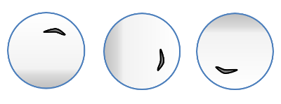
|
| 2A.R 2A.G 2A.B 2AA.R 2AA.G 2AA.B 2B.R 2B.G 2B.B 2C.R 2C.G 2C.B | RGB BGR | They are variants of features 2 that apply only to color images and work only on the specified color channel (R, G or B). These features are particularly suitable for Surface projects where the chromatic component of the defect and / or background is important for the characterization of the defects. For the other aspects they are equivalent to the original features "2". |
| 2A_RI.R 2A_RI.G 2A_RI.B 2AA_RI.R 2AA_RI.G 2AA_RI.B 2B_RI.R 2B_RI.G 2B_RI.B 2C_RI.R 2C_RI.G 2C_RI.B | RGB BGR | Variations of chromatic features invariant to rotation, indicated for Surface projects when the defect or background can take on different rotations. 
|
| Category "3" | ||
| 3A 3B 3C 3D 3E | RGB BGR | Analyze color hue and saturation without considering luminance. It is used to distinguish between objects with different colors. The spectrum of visible light, from blue to red, is divided into an histogram of 16, 32, 64, 128, 256 bins respectively for feature 3A, 3B, 3C, 3D, 3E, so the feature manages to separate quite different colors, not shades of color. The image below shows the case of feature 3A with 16 bins. 
|
| BW | From version 1.8.1 onwards features "3" can also be used on BW images. In this case the luminance is used. | |
| Category "4" | ||
| 4A | BW RGB BGR | It analyzes the local contrast level based on the luminance in the case of grayscales images and based on the chromatic components in the case of color images. It could be used together with features "2" in Surface projects, but it is not advisable to use it alone as it is not sufficiently characterizing. |
This section gives some guidelines for choosing the features for the Retina and Surface projects.
Retina project
The guidelines for choosing features for Retina can be the following:
A flow chart for Retina training could be the following:
Surface projects
The guidelines for choosing features for Surface can be the following:
The most important features for Surface are all those of category "2" which are the most suitable for modeling the texture of the surface. In fact, the default features for Surface are the "2" in the "variant to rotation" version:
Features 2A, 2B and 2C use luminance while all the others are the respective chromatic versions that work on a single color channel R, G, B.
To choose between variant or invariant features, the following scheme may be useful:
| Significant dataset | Defects of any orientation | Background of any orientation | Features | |
|---|---|---|---|---|
| 1 | YES | YES | YES | Variants/Invariants |
| 2 | YES | NO | YES | Variants/Invariants |
| 3 | YES | YES | NO | Variants/Invariants |
| 4 | YES | NO | NO | Variants |
| 5 | NO | YES | YES | Invariants |
| 6 | NO | YES | NO | Invariants |
| 7 | NO | NO | YES | Invariants |
| 8 | NO | NO | NO | Variants/Invariants |
"Defect of any orientation" it means a shape that has a main axis, for example a scratch, and that does not have specific directions but can have any angle.
"Background of any orientation" it means the presence of a texture that has a directionality and that can have any angle.
The criterion could be that, you start with the default features "variant to rotation", unless you are in cases 5, 6, 7, so preferably you start with the fetaures "invariant to rotation".
In the other cases, you start with the "variants" and only when the results are poor are the "invariants" tested.
A flow chart for Surface training could be the following:
Another criterion for choosing the features to be used in the project is the processing speed. When the machine's cycle time is critical and you need to reduce the execution time of the sb_project_detection function as much as possible you can set the sb_t_svl_sl_par::optimization_mode parameter to the SB_SVL_PAR_OPTIMIZATION_USE_SELECTED value so you can choose exactly the fastest features that suit your application. As explained in the How SB works chapter, the analysis basically consists of two parts: the extraction of the features and their classification. The extraction and classification time of the features do not follow the same trend, so there are features that require less time for extraction but more time for classification and vice versa. Furthermore, as the implementation of the features is different for BW and color images, their times are also different for BW and color images.
Below are two tables, one for BW images and the other for color images, with the intent of giving a useful indication for the choice of features based on execution times. Since it is not possible to give absolute execution times, then it has been indicated as an increase compared to the faster feature that is taken as a reference. These data were obtained by averaging the results of the many different projects. it is emphasized that these data are only indicative and that it may be that with your project different results are obtained so it is always necessary to carry out verification tests.
Features are sorted by increasing runtimes.
In the following table for gray level images:
| Feature extraction | Speed factor | Feature classification | Speed factor |
|---|---|---|---|
| 2A | x 1.0 | 2B_RI | x 1.0 |
| 2B | 2A_RI | ||
| 2A_RI | x 1.5 | 2C_RI | |
| 2B_RI | 0A | x 1.5 | |
| 0A | 0A_RI | ||
| 0B | 2A | ||
| 0B_RI | 2B | ||
| 0A_RI | 0B | ||
| 2D | x 2.5 | 0B_RI | |
| 2C | 2D | x 2.5 | |
| 2C_RI | x 3.0 | 2C |
In the following table for color images:
| Feature extraction | Speed factor | Feature classification | Speed factor |
|---|---|---|---|
| 3A | x 1.0 | 2B_RI.B | x 1.0 |
| 2A.R | x 2.5 | 2B_RI.G | |
| 2B.B | 2A_RI.R | ||
| 2AA.R | 2B_RI | ||
| 2AA.B | 2B_RI.R | ||
| 2AA.G | 2A_RI.B | ||
| 2A.B | 2A_RI.G | ||
| 2B.R | 2AA_RI.B | ||
| 2B | 2A_RI | ||
| 2A.G | 2AA_RI.G | ||
| 2B.G | 2AA_RI.R | ||
| 2A | 2C_RI.B | ||
| 2AA_RI.B | x 3.5 | 2C_RI.G | |
| 2AA_RI.R | 2C_RI | ||
| 2AA_RI.G | 2C_RI.R | ||
| 2A_RI.B | x 4.0 | 0A | x 1.5 |
| 2A_RI | 0A_RI | ||
| 2A_RI.R | 3A | ||
| 2A_RI.G | 2B | ||
| 2B_RI | 2B.B | ||
| 2B_RI.G | 2AA.R | ||
| 2B_RI.B | 2A.G | ||
| 2B_RI.R | 2A.R | ||
| 2D.G | x 6.0 | 2A | |
| 2D.R | 2AA.B | ||
| 2D | 2A.B | ||
| 2D.B | 2AA.G | ||
| 2C.B | 2B.R | ||
| 2C.R | 2B.G | ||
| 2C | 0B | ||
| 2C.G | 0B_RI | ||
| 0A_RI | 2D | x 2.5 | |
| 0B | 2D.B | ||
| 0A | 2D.R | ||
| 0B_RI | 2D.G | ||
| 2C_RI.B | x 9.0 | 2C.B | |
| 2C_RI | 2C | ||
| 2C_RI.R | 2C.R | ||
| 2C_RI.G | 2C.G |
Here are some considerations on how to use the previous tables.
Even if there are multiple models, the sb_project_detection function extracts the features only once for each level of scale and then performs the classification for each model. So if there are more models it is better to prefer a feature that is faster in classification than a faster feature in extraction.
To recognize defects with Surface, the image can be processed on different levels for each model, that means models can work on different scales from the others.
In this section the levels configuration is described.
Generally the image is processed at its original scale and resolution without any resize.
There are some situations when it is convenient and more effective to process the images at different scales:
From version 1.10.0 a new functionality has been added in the SVL of Surface project which automatically chooses the scale levels starting from the size of the defects.
To enable or disable this functionality use the parameter sb_t_svl_sl_par::auto_levels .
If enabled you should not modify the sb_t_par_model::levels list of the models.
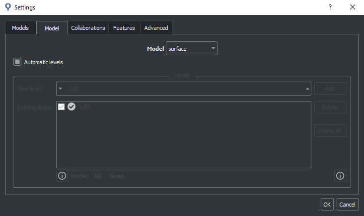
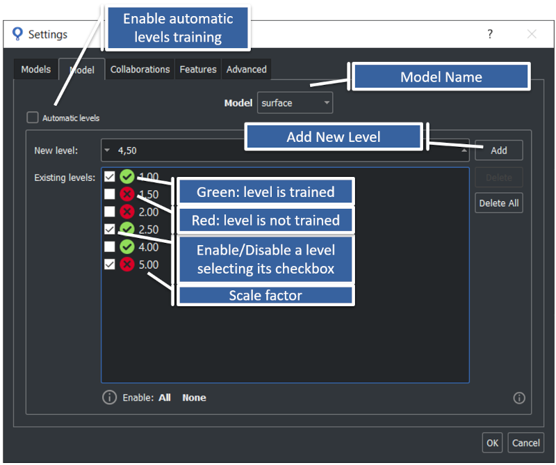
The image below shows the parameter selection in the Settings menu of the SB GUI.
The set of levels to be processed is configured with the sb_t_par_model::levels parameter and is initialized in a different way depending on the project type. See the table below.
Retina project has only 1 level because the scale is managed in another way by using the scale of the sample, see sb_t_sample::scale .
The parameter is not used by Deep Cortex and Deep Surface projects.
| Project | Predefined set of levels | Number of levels |
|---|---|---|
| Retina | 1 level at 1.0 scale | 1 fixed level at 1.0 scale |
| Surface | 0 levels | Up to 32 levels with a scale ranging from SB_PAR_LEVEL_SCALE_MIN to SB_PAR_LEVEL_SCALE_MAX |
| Deep Cortex | 0 levels (not used) | the parameter is not used and the scale is automatically managed |
| Deep Surface | 0 levels (not used) | the parameter is not used and the scale is automatically managed |
Level scales must be multiple of SB_PAR_LEVEL_SCALE_GRANULARITY and must be stored in the sb_t_par_model::levels array in ascending order. Use the functions sb_par_add_level and sb_par_remove_level to respectively add or remove a level to/from the sb_t_par_model::levels list.
These functions ensure that the list is always sorted in ascending order.
Levels configuration is only possible with Surface projects.
Level can be added with the function sb_par_add_level and removed with the function sb_par_remove_level.
To enable the automatic levels scale training do the following operations,
where sb_handle is a project handle previously loaded with the function sb_project_load or created with the function sb_project_create :
To add a level you should do the following operations, where sb_handle is a project handle previously loaded with the function sb_project_load or created with the function sb_project_create :
To remove a level you should do the following operations,
where sb_handle is a project handle previously loaded with the function sb_project_load or created with the function sb_project_create :
To disable a level of a model you should do the following operations,
where sb_handle is a project handle previously loaded with the function sb_project_load or created with the function sb_project_create :
In the SB GUI, levels for each model can ben configured for a Surface project in section Settings->Model.
SVL is the acronym for Super-Vised Learning and is the supervised procedure that carries out the training of a SqueezeBrains project using a set of labeled images.
SVL processing is composed by the following steps:
The field sb_t_svl_res::running_step is filled with the description of the current step. SVL elaborates every learning image present in the folder path specified by the parameter sb_t_svl_par::project_path and with the extension compatible with the file extensions specified by the parameter sb_t_svl_par::image_ext . An image is marked to be used for learning with the function sb_image_info_set_type.
There are 3 ways to control the training process:
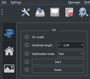
The goodness is a measure used to evaluate the training quality of Retina and Surface projects. It is an estimation of the separation between the weight or confidence of TRUE POSITIVE and TRUE NEGATIVE samples, i.e. between the foreground and the background, or, in case of Surface project, between good and defective surface. Goodness is evaluated with the equation shown below:
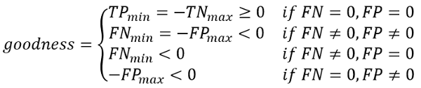
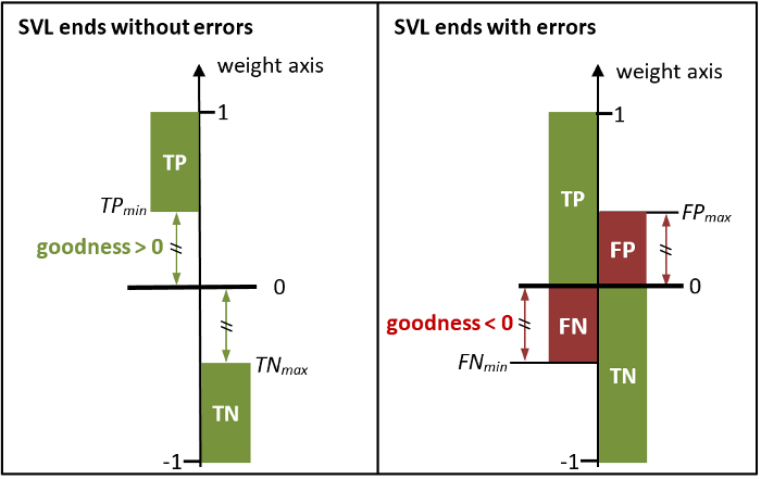
The following image shows a graphic representation of goodness. On the ordinate axis the sample weights. If training ends without errors, the zero is set exactly halfway between the set of samples TRUE POSITIVE and that of the TRUE NEGATIVE, and the goodness will be greater o equal than 0. Otherwise, if the training ends with errors (SB_TRUTH_FALSE_POSITIVE FP or SB_TRUTH_FALSE_NEGATIVE FN), the goodness will be less than 0.
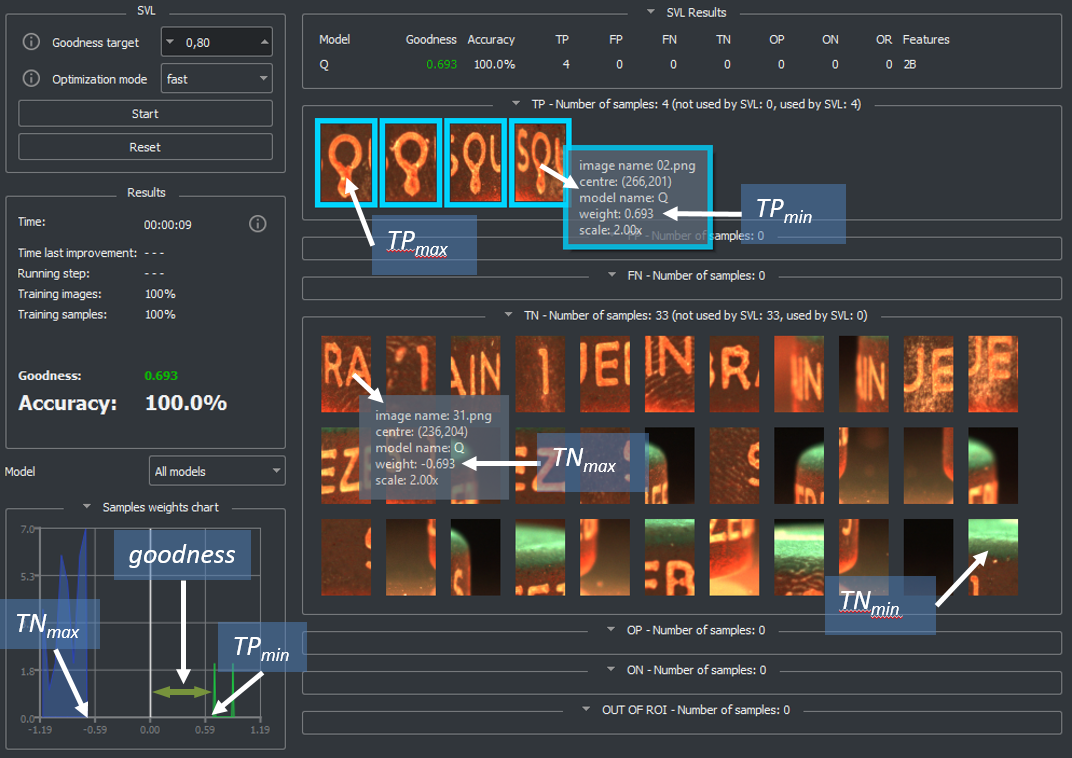
The image below shows the SVL page of the SB GUI at the end of the training. The samples are shown in descending order of weight, starting at the top left with the TRUE POSITIVE sample with the greatest weight up to the TRUE NEGATIVE sample at the bottom with the lowest weight. Only the first 100 TRUE NEGATIVE samples per model are displayed. In practice you can see an imaginary weight axis that connects all the samples and that runs from left to right and from top to bottom. If the SVL ends without errors, the TRUE POSITIVE sample with lower weight and the TRUE NEGATIVE sample with greater weight are equal in absolute value.
When the SVL starts, it loads the history from a previously saved training and uses it to proceed from that status with an incremental training. In case no SVL history is present or the function sb_svl_reset has been called, the processing starts from the beginning. The following table illustrates some specific cases and how they affect the previously saved SVL history.
| Case condition | Effect | |
|---|---|---|
| Retina/Surface | Deep Cortex/Deep Surface | |
| The models order is changed | SVL history is maintained | SVL history for all models is lost |
| A model has been disabled | SVL history for that model is maintained | SVL history for all models is lost |
| A model has been invalidated due to model parameters changes | SVL history for that model is lost | SVL history for all models is lost |
| All models has been invalidated due to parameters changes | SVL history for all models is lost | |
In order to check the current status of the SVL or to customize some behaviors and make some choices a set of callbacks is provided.
Internally, the training works on each model independently from the others. This means that the user is free to enable/disable some models before running an SVL without affecting the training results. This may be useful when it is necessary to effectively train only a subset of models, for example to speed up the training time. The user can enable/disable a specific model setting to 1/0 the flag sb_t_par_model::enabled, see the example Enable/disable a model in a project .
See sb_project_set_par for changes to other parameters that invalidate the training.
In the parameters structure sb_t_svl_par there are 3 callback pointers for a better integration of the module SVL in a custom software.
Of course is it possible to leave the callback pointers to NULL. In this case the SVL will work in the predefined mode.
The parameter sb_t_svl_par::user_data is passed to each callback so that the user can find his data inside the callback.
In the following the description of the callbacks.
The callback sb_t_svl_par::sb_fp_svl_progress is continually called to inform the caller about the progress of the SVL. For example the current accuracy.
Most of the time the callback is called only to signal to the user that the SVL is running and isn't blocked, that is, sb_t_svl_res::time_ms is increasing.
When something is changed and the user should refresh the information, the callback is called with the flag force set to 1.
The field sb_t_svl_res::running_step informs about the current step of the training.
The function sb_svl_run calls the callback sb_t_svl_par::fp_pre_elaboration for each image with type SB_IMAGE_INFO_TYPE_SVL in the folder specified with the parameter sb_t_svl_par::project_path. In the callback the user fills the sb_t_svl_pre_elaboration structure and in particular:
The SVL calls the callback sb_t_svl_par::fp_command in some different conditions:
when a particular situation happens during the learning and the SVL needs to know what the user wants to do.
In this case the parameter sb_t_svl_res::stop_reason will have the following values:
See sb_t_svl_stop_reason for more information.
The user decides the action the SVL will do with the parameter command passed to the callback. The parameter command can have the following values:
In the table below what sb_svl_run does by any combination of stop_reason and command parameters is reported.
| stop_reason \ command | SB_SVL_COMMAND_STOP | SB_SVL_COMMAND_ABORT | SB_SVL_COMMAND_CONTINUE | SB_SVL_COMMAND_CONTINUE_NO_RESET |
| SB_SVL_STOP_CONFLICT | stop | abort | continue | continue |
| SB_SVL_STOP_USER_REQUEST | stop | abort | continue | continue |
| SB_SVL_STOP_MEMORY | stop | stop | stop | stop |
| SB_SVL_STOP_RESET_MANDATORY | stop | abort | reset | reset |
| SB_SVL_STOP_RESET_OPTIONAL | stop | abort | reset | continue without reset |
| SB_SVL_STOP_WARNING | stop | abort | continue | continue |
Stop: after sb_svl_run has finished, you can call sb_project_save to save the training results.
Abort: after sb_svl_run has finished, you can not call sb_project_save to save the training results.
Perturbations is a procedure widely used in Machine Learning. It consists in generating synthetic data in order to increase the variability of instances processed by the training algorithm. Its main objective is to make the algorithm more robust on new unseen data, i.e to improve its generalization capability on test images.
In SB Library perturbations are differently implemented depending if project is of Shallow Learning or Deep Learning type.
Shallow learning perturbations are used only by Retina projects.
In this case, the perturbation is applied per model to the samples of the image. Artificial samples obtained from the perturbation are added to the original ones of the image. Depending on the parameters, a SVL perturbation generates one or more synthetic samples.
You can see the perturbations as a sequence of operations on the image of the sample.
The operations are executed in this specific order:
If you need to do only a flip you should set num_synthetic_samples equal to 1 and set angle_range equal to 0.
If you need both the sample flipped around y-axis, and the one flipped around x-axis, you should configure two perturbations, one for each flip. This solution is strongly suggested especially when the model has a symmetry, for example: horizontal, vertical or circular. If the model you want to detect has a rotation variability in a specific interval of degrees, we suggest using perturbations to make the training more robust.
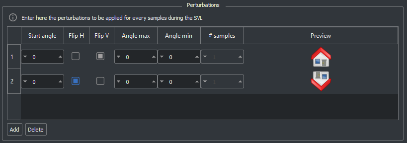
In the image below you can see the panel in the menu setting of the SB GUI. In the example below two perturbations has been added: a vertical flip and an horizontal flip.
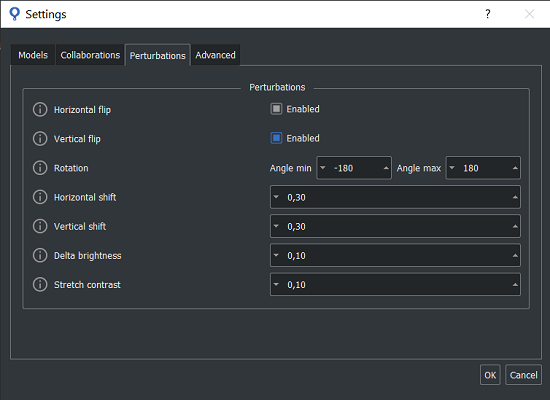
The Deep Learning perturbations are used for Deep Surface and Deep Cortex projects.
In this case a perturbation is applied during SVL to the entire training image and not to a part of this (e.g. to a sample) as in shallow learning case. In addition deep learning perturbation does not contribute to numerically increase the amount of images processed by an epoch (i.e. a loop over the entire training set), but only force to use every time a different perturbated version of the same image. When multiple perturbations are enabled, their order does not affect the gloabal perturbated image. Operations executed by perturbation may be of two types:
All deep learning perturbations are applied by default in pseudo-random way depending from the current epoch. This allow, at same condition of training images and parameters, to be sure that each image is always equally perturbated at the same epoch. For a full randomness disable sb_t_svl_par::reproducibility.
In the image below you can see the panel Perturbations where choosing deep learning perturbations in the Settings Menu of the SB GUI.
Sometime the user doesn't want to elaborate the acquired image but a warped version of it. However, he wants to show to the operator the acquired image, and he wants that the operator sets the sample on this image. So happens that the coordinates of the samples in the RTN files are referred to the acquired image while the SVL needs to have the samples referred to the warped image.
To manage correctly this situation, the SVL needs to warp the point coordinates of the samples using the lut functions.
Using these functions it is possible to create luts to map the coordinates of a point referred to the acquired image into the coordinates referred to the warped one and vice versa. The SVL will use this luts to warp the coordinates of the samples.
To use the lut the user should do the following steps.
It is possibile to create and manage a ROI (Region Of Interest) with a generic shape.
The ROI is an image with the same size of the source image.
You can set each pixel of the ROI as belonging to the ROI or not. Only the selected pixels will be elaborated.
Each pixel of the ROI is 8 bit depth.
There are two different types of ROI:
| Model | Required | Optional |
|---|---|---|
| 0 | 255 | 127 |
| 1 | 254 | 126 |
| . . . | . . . | . . . |
| 125 | 130 | 2 |
| 126 | 129 | 1 |
To check if a pixel of the image will be elaborated, the functions, for instance sb_project_detection , uses the following formula :
In order to reduce the memory usage you can call sb_roi_compress to encode the ROI with RLE (Run Length Encoding). You can use sb_roi_decompress to decode the ROI.
To create a ROI for an existing image use the following procedure
SB Library manages BW and color images with the following format:
The Image is described by the structure sb_t_image which can be created in two modes:
The function sb_image_load loads an image from file. The supported file types are:
To load an image from file use the following function:
In case the image is already in memory, it is possible to create a sb_t_image object and then connect or copy the image data pointer.
A fundamental step to configure Deep Cortex and Deep Surface projects is the selection of the computational devices to run inner operations of sb_svl_run and sb_project_detection functions. In fact, deep learning algorithms generally need a computational effort significantly higher than Retina or Surface and this may lead to long training and detection time.
A strongly recommended practice for deep learning users who want to run training is to have installed on the machine a NVIDIA GPU (Graphics Processing Unit) with CUDA support. CUDA (Compute Unified Device Architecture) is a parallel computing platform and API that allows to use GPU NVIDIA to accelerate graphics processing. Here, the official list of GPU NVIDIA marketed by NVIDIA: https://developer.nvidia.com/cuda-gpus .
For what concern detection, alongside SB_DEVICE_CPU and SB_DEVICE_GPU_NVIDIA, SqueezeBrains allows the user also to use OpenVino compatible devices. Thus, from version 1.15.0, also the following are available: SB_DEVICE_CPU , SB_DEVICE_IGPU_INTEL and SB_DEVICE_DGPU_INTEL . They run an optimized version of the algorithm and detection time is comparable to what obtained on GPU NVIDIA. It's important to note that elaboration time depends also on Deep Learning parameters set by the user.
User can recover at any time the info of devices currently available on machine with the function sb_get_info.
To set computational device for Deep Cortex or Deep Surface projects you should do the following operations,
where sb_handle is a project handle previously loaded with the function sb_project_load or created with the function sb_project_create :
If no device is set by the user, the following rule is applied:
It may happen that the selected device is not available on the machine. This can be due to the following reasons:
In all this cases no error is notified. Depending on the case the following rule is applied:
You can find useful advices for choosing the GPU for your project in the following document Guida_scelta_GPU.pdf.
The SB library has been developed to parallelize operations on multiple CPU threads. Today almost all processors have multiple cores and also hyper threading technology that makes a physical CPU appear as two logical CPUs.
Parallelizing the operations allows to reduce the calculation times.
It is difficult to predict what is the number of physical / logical processors with which you have the least calculation time because the architecture of a PC is complex and includes many other parts that are involved in the calculation and that can become bottlenecks. Consider that image processing involves a large transfer of data between memory and CPU, the greater the larger the images. So the bandwidth of the communication buses between RAM and CPU is another particularly important parameter. Furthermore, linked to this parameter, there are also the sizes of the L1, L2 and L3 caches. Of course, CPU frequency is also a determining factor.
Having made these considerations, it is clear that it is not possible to predict a priori the number of threads that minimizes the calculation time and therefore all that remains is to do tests.
A good compromise is a number of threads equal to the physical number of cores of a CPU, but this is not always the best value. Usually the greatest reduction occurs when going from 1 to 2 threads then, adding more threads the time reduction is always lower up to the point where, instead of decreasing, the time increases again. The increase in time is mainly due to the congestion of the communication buses and the L1, L2 and L3 caches.
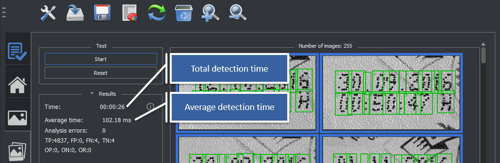
The procedure we recommend to optimize the number of threads is to start from 1 thread and increase the value of 1 thread at a time: for each thread value you must run a test on a set of images whose total processing time is greater than 10 s (this because the processors go into power save mode and take a while to return to the nominal speed). The optimal thread value is the one that minimizes computation time.
As shown in the image below, the SB GUI, in the test section, shows both the total detection time and the average detection time.
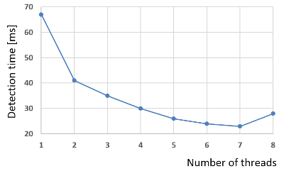
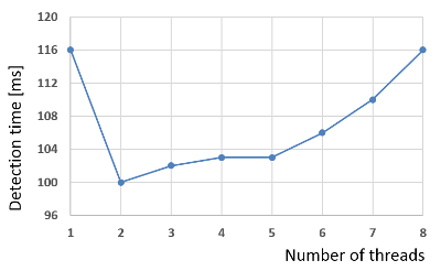
The following image shows two examples. The test was done on an i7-4710HQ processor which has 4 physical hyper threading cores for which 8 logical Cores. In the first example the number of threads that minimizes the detection time is 7 while in the second is 2.
For the library to be used in all its functions it is necessary to have an active license.
There are three different license:
In order to modulate the price of the license, 3 configurations have been created, basic, standard and Premium. The Basic configuration is the cheapest but the most limited, the Premium configuration is the most expensive but has no limitations. The configuration are based on the following parameters:
| parameter | Description | ||||||||||||
|---|---|---|---|---|---|---|---|---|---|---|---|---|---|
| Training | It indicates if training is enabled or not. If it is not enabled the function sb_svl_run will return the error SB_ERR_LICENSE_TRAINING. | ||||||||||||
| Number of models | It is the maximum number of models that can be set in the sb_t_par structure. The functions sb_svl_run and sb_project_detection will return the error SB_ERR_LICENSE_MODELS_NUMBER if the project has more models than the maximum allowed by the license configuration. | ||||||||||||
| Number of features | Only for Retina and Surface modules. It is the maximum number of features that the SVL can choose automaticaly. See Features to know how to configure the set of features. The function sb_svl_run will return error if mode SB_SVL_PAR_OPTIMIZATION_USE_SELECTED is set in the structure sb_t_svl_par and, in the set of features, there are more than those allowed by the license configuration. The function sb_project_detection will return the error SB_ERR_LICENSE_FEATURES_NUMBER is the project has more features than those allowed by the license configuration. | ||||||||||||
| Speed | It has 3 levels: slow, medium, fast.
Both the parameters are in the structure sb_t_par.
The functions sb_svl_run and sb_project_detection will not return error if you set speed_boost and / or num_threads with a value greater than the maximum allowed by the license configuration, but they limit the parameters to the maximum allowed value.
|
The following table shows all the properties of the configurations.
| Configuration | License module | Training | Number of models | Number of features | Speed | Description |
|---|---|---|---|---|---|---|
| Basic | Retina runtime | no | 1 | 1 | slow | Basic Retina runtime |
| Retina | yes | 1 | 1 | slow | Basic Retina | |
| Surface runtime | no | 1 | 3 | slow | Basic Surface runtime | |
| Surface | yes | 1 | 3 | slow | Basic Surface | |
| Deep Cortex runtime | no | 1 | not used | slow | Basic Deep Cortex runtime | |
| Deep Cortex | yes | 1 | not used | slow | Basic Deep Cortex | |
| Deep Surface runtime | no | 1 | not used | slow | Basic Deep Surface runtime | |
| Deep Surface | yes | 1 | not used | slow | Basic Deep Surface | |
| Deep Retina runtime | no | 1 | not used | slow | Basic Deep Retina runtime | |
| Deep Retina | yes | 1 | not used | slow | Basic Deep Retina | |
| Standard | Retina runtime | no | 5 | 3 | medium | Standard Retina runtime |
| Retina | yes | 5 | 3 | medium | Standard Retina | |
| Surface runtime | no | 3 | 6 | medium | Standard Surface runtime | |
| Surface | yes | 3 | 6 | medium | Standard Surface | |
| Deep Cortex runtime | no | 5 | not used | medium | Standard Deep Cortex runtime | |
| Deep Cortex | yes | 5 | not used | medium | Standard Deep Cortex | |
| Deep Surface runtime | no | 3 | not used | medium | Standard Deep Surface runtime | |
| Deep Surface | yes | 3 | not used | medium | Standard Deep Surface | |
| Deep Retina runtime | no | 5 | not used | medium | Standard Deep Retina runtime | |
| Deep Retina | yes | 5 | not used | medium | Standard Deep Retina | |
| Premium | Retina runtime | no | 64 | unlimited | fast | Premium Retina runtime |
| Retina | yes | 64 | unlimited | fast | Premium Retina | |
| Surface runtime | no | 64 | unlimited | fast | Premium Surface runtime | |
| Surface | yes | 64 | unlimited | fast | Premium Surface | |
| Deep Cortex runtime | no | 64 | not used | fast | Premium Deep Cortex runtime | |
| Deep Cortex | yes | 64 | not used | fast | Premium Deep Cortex | |
| Deep Surface runtime | no | 64 | not used | fast | Premium Deep Surface runtime | |
| Deep Surface | yes | 64 | not used | fast | Premium Deep Surface | |
| Deep Retina runtime | no | 64 | not used | fast | Premium Deep Retina runtime | |
| Deep Retina | yes | 64 | not used | fast | Premium Deep Retina |
A license includes up four modules, also with different configurations.
You can use the function sb_license_get_info to get information about your current license configuration.
The license is initialized by the function sb_init.
Once the sb_init is finished, the license may not yet be initialized so if the sb_svl_run or sb_project_detection function is called immediately it would give the error SB_ERR_LICENSE. So, after the sb_init function, you need to wait for the license to be validated by calling the function sb_license_get_info in a loop. See the tutorial init_library.c as an example of initialization. In particular, see the function wait_license, that waits for the license to become active.
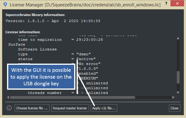
When you receive the dongle USB key it will be empty, with no license enabled.
Together with the dongle you will also receive a file with v2c extension (Vendor to Customer) that will be used to enable the licenses you have purchased.
You can use the function sb_license_apply_v2c to apply the v2c file to the dongle, or you can also use the SB GUI as shown in the image below.
When you create a project you can also know which license configuration you need.
The function sb_license_configuration_check checks if your project is compatible with a certain configuration.
The compatibility only affects the functions sb_svl_run and sb_project_detection .
There are two levels of compatibility:
See also the tutorial check_license_configuration.c for more information
In the example below how to check the license configuration compatibility of a project: