sb_t_sample_weights_image Struct Reference

Image of weights of the sample. More...

#include <sb.h>

Collaboration diagram for sb_t_sample_weights_image:

Data Fields
sb_t_image *	img
	Image of the weights of the sample, format is SB_IMAGE_FORMAT_BW8.
float	max
	maximum weight corresponding, in the image, the to value 255.
float	min
	minimum weight corresponding, in the image, the to value 1.

Detailed Description

Image of weights of the sample.

Image has the same resolution as the sample size (sb_t_retina_par.model.obj_size) and is a gray scale rappresentation of the prediction weight in each pixel of the sample, where

• 128 corresponds to the weight zero
• 255 is the maximum weight equal to the field max
• 1 is the minimum weight equal to the field min
• 0 weight not evaluated

The weights map has been exported for two main purpouse:

1. Background Foreground misunderstanding
   It is very useful to be able to check if the classifier has correctly understood which object is to be recognized and therefore segmented with respect to the background. In fact, it can happen that the classifier gets confused and trains on the background instead of on the object. This problem is all the more critical the smaller the percentage of the object area compared to that of the whole sample, ie obj_size. For example, L-shaped objects or ring objects, where the most part of the sample area is occupied by the background.
   Generally if the background has a low degree of variability in the dataset, may be happen that the classifier learns to describe the model depending by the background information and not by the object one.
   To avoid this problem it is advisable to acquire images of the objects by varying the background.
   The areas of the sample that belong to the foreground must have a value from 128 to 255, shown from transparent to green by SB GUI, while those belonging to the background must have a value from 1 to 127, shown from transparent to red by SB GUI.
   In the example below the classifier has been trained to detect wheels. In the following example the classifier has been trained to detect the wheels. As you can see, the foreground, the wheel in this case, is almost completely green, while the background is almost all transparent or red. Note the area at the bottom right of the sample where the road surface is seen. It is green because in the training samples, in this corner of the sample, the road surface was always present, so the classifier, rightly, learned that the presence of the road surface in this area of the sample is correct and the prediction weight is positive. On the other hand, the lower left corner, where the road surface is not visible, is red.
   

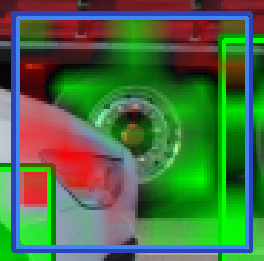
   Weights map of the a sample

   See also

   Misclassification errors

2. Detection of bad sample in semi-supervised mode
   In certain particular conditions it is possible to use Retina as a tool to separate the good pieces from the rejected ones in an unsupervised way. The weight map allows you to identify the defective part of the object represented by the pixels that have a value ranging from 1 to 127, shown in red in the SB GUI.

   See also

   How to use Retina to sort good and bad samples.

Definition at line 8101 of file sb.h.

---

The documentation for this struct was generated from the following file:

• sb.h